Dynamic Bernstein-Vazirani using mid-circuit reset and measurement#
The ability to do mid-circuit reset and measurement unlocks a variety of tools for executing quantum circuits. A brief discussion is given in this IBM Research blog post. On particular possibility is the ability to reuse qubits, and in doing so reduce the hardware requirements of some algorithms. The Bernstein-Vazirani (BV) algorithm is one such example. In particular, when using phase-kickback, BV usually requires a high degree of qubit connectivity to impliment. This has been used by trapped-ion hardware vendors to show that their hardware gives better fidelity on these problems, e.g. see (https://arxiv.org/abs/2102.00371 and https://www.nature.com/articles/s41467-019-13534-2). However, with reset and measurement, BV requires only two qubits, making connectivity differences mute. We showed this in a reply Tweet: https://twitter.com/nonhermitian/status/1362348935440986113, but did not explain how we got that figure. So here is how I did it.
Frontmatter#
import numpy as np
from qiskit import *
from qiskit.quantum_info import hellinger_fidelity
import matplotlib.pyplot as plt
import seaborn as sns

sns.set_style('darkgrid')
IBMQ.load_account()
<AccountProvider for IBMQ(hub='ibm-q', group='open', project='main')>
Select the target backend#
Here we select the backend and extract its two-qubit gate coupling map. This is not the same backend used in the original figure as, at the time or writing, that one is offline. It is however the same processor family and revision.
provider = IBMQ.get_provider(project='internal-test')
backend = provider.backend.ibm_cairo
cmap = backend.configuration().coupling_map
Create circuits#
In BV each qubit corresponding to a ‘1’ bit interacts with only the target qubit. Moreover, since the state of the target qubit is an eigenstate of the x operator, the qubits remain unentangled, and the whole algorithm can be written using only two qubits provided that those qubits can be measured and reset mid-circuit. The function below will create the circuit that does this for a given input bitstring:
def bv_circ(bitstring):
    """Create a Bernstein-Vazirani circuit from a given bitstring.

    Parameters:
        bitstring (str): A bitstring.

    Returns:
        QuantumCircuit: Output circuit.
    """
    qc = QuantumCircuit(2, len(bitstring))
    qc.x(1)
    qc.h(1)
    for idx, bit in enumerate(bitstring[::-1]):
        qc.h(0)
        if int(bit):
            qc.cx(0, 1)
        qc.h(0)
        qc.measure(0,idx)
        qc.barrier([0,1])
        qc.reset(0)
        # reset control
        qc.reset(1)
        qc.x(1)
        qc.h(1)

    return qc
Finding the best two-qubits to use#
Let us look at an example circuit for a length 10 bitstring of all ones:
bitstring = '1'*10

qc = bv_circ(bitstring)
qc.draw('mpl')

One can see that one qubit q0 there are repeated measurement+reset operations that take place. Every reset is itself a measurement followed by a conditional x-gate. Therefore we are doing two measurements back-to-back each time we see that combination of operations. Doing measurements like this can lead to issues. Namely, for example, if the measurement cavity ring-down time is not short enough, the cavity could be non-empty the next time one performs a measurement and things can get messy. It turns out to actually be a bit more complicated than that, so at the end of the day, we need to figure out which qubits are the best to us. Here we will do that by performing a 10-digit BV experiment on every edge of the systems two-qubit coupling map. We will take whichever one gives the best result as the edge to use for the actual experiment.
circs = []
for edge in cmap:
    trans_qc = transpile(qc, backend, initial_layout=edge)
    circs.append(trans_qc)
job = execute(circs, backend, shots=8192)
Here we compute the fidelity of the output with the known answer to see which gets the closest and sort the results from best to worse in terms of the fidelity.
fids = [hellinger_fidelity(counts, {bitstring: 1}) for counts in job.result().get_counts()]
sorted_fidelities, sorted_edges = zip(*sorted(zip(fids, cmap), reverse=True))
for idx, edge in enumerate(sorted_edges):
    print(edge, sorted_fidelities[idx])
[12, 10] 0.787109375
[15, 12] 0.7611083984375
[21, 18] 0.7478027343749999
[5, 8] 0.7426757812499999
[10, 12] 0.7342529296875
[14, 11] 0.7335205078125001
[18, 17] 0.732177734375
[11, 14] 0.7274169921875001
[11, 8] 0.7211914062500001
[15, 18] 0.7196044921875
[17, 18] 0.7133789062499999
[12, 13] 0.7061767578125
[8, 5] 0.6993408203125001
[2, 3] 0.6868896484375001
[8, 11] 0.6839599609375001
[13, 14] 0.6837158203125
[14, 13] 0.683349609375
[9, 8] 0.6793212890625
[23, 24] 0.6715087890625
[24, 25] 0.6627197265625001
[5, 3] 0.6622314453125001
[22, 19] 0.6545410156250001
[13, 12] 0.6502685546875
[4, 1] 0.650146484375
[19, 22] 0.6381835937500001
[10, 7] 0.6345214843750001
[20, 19] 0.6341552734375
[19, 20] 0.6315917968750002
[7, 10] 0.6259765625000001
[8, 9] 0.6256103515625001
[14, 16] 0.6195068359375
[1, 4] 0.608154296875
[0, 1] 0.6065673828125001
[22, 25] 0.6042480468750002
[7, 4] 0.5914306640625001
[2, 1] 0.5823974609375001
[3, 5] 0.579833984375
[1, 0] 0.578369140625
[3, 2] 0.56298828125
[25, 24] 0.5587158203125001
[26, 25] 0.5572509765624999
[25, 22] 0.5478515625000001
[7, 6] 0.5463867187500001
[16, 14] 0.540771484375
[18, 21] 0.5361328124999999
[1, 2] 0.5299072265625
[25, 26] 0.5206298828125
[24, 23] 0.5153808593750001
[21, 23] 0.5070800781250001
[16, 19] 0.48986816406250006
[23, 21] 0.46118164062499994
[19, 16] 0.38427734375000006
[12, 15] 0.35766601562500006
[18, 15] 0.34863281250000017
[4, 7] 0.20458984375000003
[6, 7] 0.14062500000000008
We can see from above that there is a very wide range of fidelities that come out. This just goes to show that, when doing this on today’s hardware, the choice of qubits matters quite a bit. Having found the optimal edge on which to run, we now use that to do extended BV circuit runs.
Run actual experiment#
Here we choose a set of bitstring lengths to run and then execute this on the target backend edge that we identified earlier as the best candidate. For fun, we will also run on the worst edge to see the difference.
bit_lengths = [1, 5, 10, 15, 20, 25, 30]

circs = [bv_circ('1'*kk) for kk in bit_lengths]
trans_circs_best = transpile(circs, backend, initial_layout=sorted_edges[0])
trans_circs_worst = transpile(circs, backend, initial_layout=sorted_edges[-1])
job2 = execute(trans_circs_best, backend, shots=8192)
job3 = execute(trans_circs_worst, backend, shots=8192)
fids_best = []
fids_worst = []
for idx, counts in enumerate(job2.result().get_counts()):
    fids_best.append(hellinger_fidelity(counts, {'1'*bit_lengths[idx]: 1}))

for idx, counts in enumerate(job3.result().get_counts()):
    fids_worst.append(hellinger_fidelity(counts, {'1'*bit_lengths[idx]: 1}))
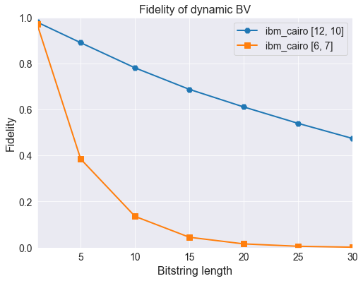
Plot results#
label_best = "{} {}".format(backend.name(), sorted_edges[0])
label_worst = "{} {}".format(backend.name(), sorted_edges[-1])

fig, ax = plt.subplots(figsize=(8,6))
ax.plot(bit_lengths, fids_best, 'H-', label=label_best, lw=2, ms=8)
ax.plot(bit_lengths, fids_worst, 's-', label=label_worst, lw=2, ms=8)
ax.set_xlabel('Bitstring length', fontsize=16)
ax.set_ylabel('Fidelity', fontsize=16)
ax.set_xlim([1, 30])
ax.set_ylim([0, 1])
ax.set_title('Fidelity of dynamic BV', fontsize=16)
ax.legend(fontsize=14)
ax.tick_params(axis='both', labelsize=14);