Comparison of Falcon R5 processors verse R4

Recently IBM Quantum announced the move to revision 5 (R5) of its Falcon processors see this tweet from Jay Gambetta. In particular it was highlighted that there is a 8x reduction in meausrement time on these systems. Lets see if this, or any other enhancements, are visible from the system calibration data.

Summary

The highlight of the recently released Falcon R5 “core” systems is their much improved measurement times (7x) and error rates (2x). On these systems a measurement is roughly twice as long as a CNOT gate, compared to 13x on the old R4 systems, and allows for implimenting high-fidelity dynamic circuits with resets, mid-circuit measurements, and eventually classically-conditioned gates. For other tasks, the modest improvements in the CNOT gate errors and \(T_{1}\) times are also welcomed.

Frontmatter

import numpy as np
from qiskit import *

import matplotlib.pyplot as plt
plt.style.use('nonhermitian')

Load account and backend selection

Loading account and making two lists; one for R5 backends and the other for R4. Which is which can be found on the systems page.

IBMQ.load_account();

provider = IBMQ.get_provider(project='internal-test')

r5_backends = ['ibmq_kolkata', 'ibm_hanoi', 'ibm_kawasaki', 'ibm_cairo', 'ibm_auckland']

r4_backends = ['ibmq_montreal', 'ibmq_dublin', 'ibmq_toronto', 'ibmq_sydney']

Get the calibration data

Here we make a function to get the calibration data and grab the results for our targeted machines.

def backends_data(backends):
    """Return backend calibration data for a list of backends.
    
    Parameters:
        backends (list): A list of backend names.
        
    Returns:
        list: cx gate errors
        list: cx gate times
        list: meas errors
        list: meas times
        list: T1 values
        list: T2 values
    """
    cx_gate_errors = []
    cx_gate_times = []
    meas_errors = []
    meas_times = []
    t1s = []
    t2s = []

    for back in backends:
        backend = provider.get_backend(back)
        props = backend.properties()
        for gate in props.gates:
            if 'cx' in gate.name:
                if gate.parameters[0].value != 1.0:
                    cx_gate_errors.append(gate.parameters[0].value)
                cx_gate_times.append(gate.parameters[1].value)

        for qubit in props.qubits:
            for item in qubit:
                if item.name == 'readout_error':
                    meas_errors.append(item.value)
                elif item.name == 'readout_length':
                    meas_times.append(item.value)
                elif item.name == 'T1':
                    t1s.append(item.value)
                elif item.name == 'T2':
                    t2s.append(item.value)
                    
    return cx_gate_errors, cx_gate_times, meas_errors, meas_times, t1s, t2s

r5_data = backends_data(r5_backends)
r4_data = backends_data(r4_backends)

Plot results

Here we compute the improvement of R5 over R4, if any, and plot it in a bar plot.

improve = [np.median(r4_data[kk])/np.median(r5_data[kk]) for kk in range(4)]
improve.extend([np.median(r5_data[-2])/np.median(r4_data[-2]),
                np.median(r5_data[-1])/np.median(r4_data[-1])])

names = ['cx_error', 'cx_speed', 'meas_error', 'meas_speed',
         '$\mathrm{T}_{1}$', '$\mathrm{T}_{2}$']

fig, ax = plt.subplots(figsize=(8,6))
bars = ax.barh(names, improve)
ax.axvline(1, color='0.3', linestyle='dashed', lw=2)
ax.set_title('Falcon R5 characteristics verses R4')
ax.set_xlabel('Improvement')
ax.set_xlim([0, 8])
for bar in bars:
    width = bar.get_width()
    plt.text(bar.get_width()+0.3, bar.get_y()+0.5*bar.get_height(),
             '%sx' % np.round(width, 1),
             ha='center', va='center',fontsize=12, weight="semibold", color='0.3')

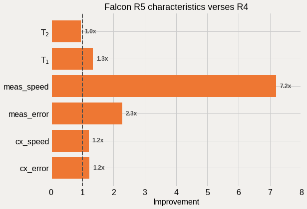
Ok cool, we do indeed see a roughly 7x improvment in the median measurement time, as well as an over 2x reduction in the associated measurement error. Not only that, there is a modest improvement in the CNOT gate speed and error rates as well, with a bit better \(T_{1}\) to round out the gains. How was this accomplished? Well the measurement gains come from a combination of increased measurement cavity linewidth (\(\kappa\)) due to stronger coupling, as well an increased in the dispersive shift (\(\chi\)) that aids in visibility. The improvements in the CNOT gates comes from further refinements in how the gates are performed.

This reduction in measurement time, and error, is critical for implimenting dynamic circuits with qubit reset, mid-circuit measurements, and eventually conditional logic. Ideally, measurement should not take any longer than any gate, and we can look to see how the R5 measurement times compare to the CNOT gate times:

print('Median R5 CNOT gate time:  ', np.median(r5_data[1]))
print('Median R5 measurement time:', np.median(r5_data[3]))

Median R5 CNOT gate time:   348.4444444444444
Median R5 measurement time: 732.4444444444445

We see that a measurement takes about twice as long as a CNOT gate on the R5 systems. Thus, the R5 systens achieve the goal of high-fidelity readout on a timescale no longe than the typical gate times on the system. What about the old R4 systems?

print('Median R4 CNOT gate time:  ', np.median(r4_data[1]))
print('Median R4 measurement time:', np.median(r4_data[3]))

Median R4 CNOT gate time:   419.55555555555554
Median R4 measurement time: 5276.444444444443

Ouch! Each CNOT gate on an R4 system is roughly 13 CNOT gates in terms of time. Not a good situation to be in when you need to measure and reset a qubit mid-circuit. Indeed, trying to do so on the R4 systems quickly leads to headaches. For example, you can try to play with the dynamic Bernstein-Vazirani example using an R5 (as done there) and comparing it to an R4 system.

Choosing the best Qiskit swap mapper   Excited State Promotion (ESP) Readout