Excited State Promotion (ESP) Readout#
Summary#
Excited State Promotion (ESP) readout is method for decreasing measurement errors in quantum computing systems where decay from the excited \(|1\rangle\) state to \(|0\rangle\) is non-negligible over the measurement timescales. Although it was originally an useful technique on the previous generation Falcon R4 systems, today it is only available on a few Falcon R5 systems where the nearly order of magnitude improvement in measurement times leaves little value in using this functionality. In testing, it looks to even be a bit worse performing than the standard readout method. ESP readout is on by default for those systems that support it. To disable it run:
backend.run(circs, use_measure_esp=False)
Background#
On many quantum computing platforms one of the two computational basis states, the \(|1\rangle\) state by convention, is an excited state of the system with respect to the ground state \(|0\rangle\). The difference in energy between these two states defines the frequency of the qubit through the relation \(E=hf\). Because the \(|1\rangle\) state is an excited state, there is a non-zero probability that the state will decay to \(|0\rangle\) via interaction with the environment. The characteristic timescale for this is the \(T_{1}\) time of the qubit. When performing gate operations, or non-reversible instructions like measurements on qubits, if the time it takes to perform these operations is a non-negligible fraction of \(T_{1}\), then there is a possibility that this decay has occurred.
Earlier we looked that the difference between Falcon R5 and R4 systems and saw that on the earlier R4 devices measurements took an amount of time equivalent to 13 CNOT gates on average. This is quite a long time, and given our discussion above, we would expect that a qubit in the \(|1\rangle\) state would have a non-negligible probability of decaying into the ground state during this time; our measurement of the \(|1\rangle\) state would incur some error from this decay process. Indeed this is what happens. While all qubit measurements have some associated error, there is an asymmetry between the error rates of measuring the \(|0\rangle\) and \(|1\rangle\) states due to this effect, and the error associated with measuring the \(|1\rangle\) state are typically larger than those of the ground state. As such, finding a method to minimize the error associated with this environmentally induced decay would lead to higher-fidelity measurements on IBM Quantum systems and beyond.
Excited State Promotion (ESP) readout is one such method to reduce this error. To understand how this works we first note that qubit measurements tell you only two things; Is the qubit in the ground state, or is the qubit in any other state? That is it. The readout does not care if your in the \(|1\rangle\) state the \(|2\rangle\) state etc. ESP readout takes advantage of this in the following way. If I “promote” the \(|1\rangle\) state of the qubit to the \(|2\rangle\) state (of what is now a qudit since it is no longer two-levels) then my measurement is unaffected. However what is affected is the timescale over which my qudit will decay into the \(|0\rangle\) state. In the standard regime where single-photon processes are dominant, a qudit starting in the \(|2\rangle\) state must first decay into the \(|1\rangle\) state before decaying into the \(|0\rangle\) state. Because each of these processes has a timescale associated with it, and our measurement does not care about the difference between \(|2\rangle\) and \(|1\rangle\) we have gained some amount of time before our measurement is affected by the decay; Our measurement fidelity should be improved. The benefit of this method was demonstrated on the Falcon R4 ibmq_montreal system when looking at Quantum Volume. However, on newer systems, with their ~7x improvement in measurement time, the utility of this method has not been addressed. Here we will look to see what, if any, value this technique has.
Frontmatter#
import numpy as np
import mthree
from qiskit import *

import matplotlib.pyplot as plt
#plt.style.use('ibmq-dark')
%config InlineBackend.figure_format='retina'
Here we are importing some tools from M3 that are not really user facing, but are useful here.
from mthree.mitigation import _balanced_cal_strings, _balanced_cal_circuits
Load account and backend selection#
In order to play around with ESP readout we first need to find out which systems support it. This is done by querying the system configuration for the 'measure_esp_enabled' attribute. Since this attribute need not be present at all, we need to be a bit careful and use a try-except block or, as done here, getattr:
IBMQ.load_account();
provider = IBMQ.get_provider(project='internal-test')
for _backend in provider.backends():
    if getattr(_backend.configuration(), 'measure_esp_enabled', False):
        print(_backend.name())
ibm_bangkok
ibm_hanoi
ibm_cairo
ibm_perth
Although I have access to every IBM Quantum system out there, it turns out that only 4 of them actually have ESP readout enabled, and they are all R5 systems. I am not sure why the ibmq_montreal system does not have it enabled given that that was the first system that had it. Unfortunately what this means is that we cannot evaluate what benefit ESP has on the older R4 systems. I am assuming it probably helped a fair bit, but we cannot prove it. Here we will pick on of the R5 systems.
backend = provider.backend.ibm_cairo
Balanced calibrations#
We aim to look at the difference in error rates when using ESP readout and those with it disabled. To do that we need to determine these error rates through calibration. There are many ways to calibrate measurement errors. We could prep each qubit individually in either the \(|0\rangle\) or \(|1\rangle\) state and sample the resulting output to determine the error rates (\(2N\) circuits in total where \(N\) is the number of qubits on the system). Alternatively, as done in Qiskit Ignis, we could prep just two states the \(|00\dots 0\rangle\) and \(|11\dots 1\rangle\) and take marginal counts. While both are valid, they do have their downsides. The first method treats each qubit individually, but is not very efficient. The latter technique is very efficient, but is quite sensitive to state preparation errors, if they exist.
Here we will use an alternative created created by yours truly for obtaining very accurate error rates while trying to minimize sensitivity to things like state-prep errors. This “balanced” calibration method works by executing bit-strings with a pattern that allows for sampling each error rate \(N*\rm shots\) times in a manner that is not particularly biased in terms of sensitivity to state-prep errors. Thus, for the same amount of work as doing each qubit individually, we get a factor of \(N\) enhancement in the number of samples per error rate while not being sensitive to state prep errors along a particular basis direction. We can generate these balanced calibration strings and generate the circuits.
num_cal_qubits = backend.configuration().num_qubits
cal_strings = _balanced_cal_strings(num_cal_qubits)
Lets take a look at a subset of balanced calibration strings:
cal_strings[:6]
['010101010101010101010101010',
 '101010101010101010101010101',
 '001100110011001100110011001',
 '110011001100110011001100110',
 '000111000111000111000111000',
 '111000111000111000111000111']
We now convert these strings to our calibration circuits:
circs = _balanced_cal_circuits(cal_strings)
Experiments#
We now perform our experiments running the balanced calibration routine with and without ESP readout. Here we use \(10000\) shots per circuit giving us an effectively sampling per error rate of \(270,000\) shots. So our results should be pretty good. To turn ESP on and off we need to use the use_measure_esp keyword argument in backend.run(). When available, ESP readout is enabled by default. The code below is mainly taken from the M3 source code for doing the marginalization over the balanced calibration data. The important part is that the results with and without ESP are stored in cal_result, in that order.
cal_shots = 10000
cal_results = []

for use_esp in [True, False]:
    job = backend.run(circs, shots=cal_shots, use_measure_esp=use_esp)
    counts = job.result().get_counts()

    cals = [np.zeros((2, 2), dtype=float) for kk in range(num_cal_qubits)]
    for idx, count in enumerate(counts):

        target = cal_strings[idx][::-1]
        good_prep = np.zeros(num_cal_qubits, dtype=float)
        denom = cal_shots * num_cal_qubits

        for key, val in count.items():
            key = key[::-1]
            for kk in range(num_cal_qubits):
                if key[kk] == target[kk]:
                    good_prep[kk] += val

        for kk, cal in enumerate(cals):
            if target[kk] == '0':
                cal[0, 0] += good_prep[kk] / denom
            else:
                cal[1, 1] += good_prep[kk] / denom

    for jj, cal in enumerate(cals):
        cal[1, 0] = 1.0 - cal[0, 0]
        cal[0, 1] = 1.0 - cal[1, 1]

    cal_results.append(cals)
The diagonal of the calibration matrix tells us the fidelity of the measurement process per qubit. Here we take the average over the fidelities for the \(|0\rangle\) and \(|1\rangle\) states.
esp_fids = [np.array([np.mean(q.diagonal()) for q in cals]) for cals in cal_results]
It is easier to look at the error rates (but easier to extract the fidelities) so we plot those for each qubit.
fig, ax = plt.subplots()
ax.bar(np.arange(num_cal_qubits), 1-esp_fids[0], width=0.33, label='ESP active')
ax.bar(np.arange(num_cal_qubits)+0.33, 1-esp_fids[1], width=0.33, label='ESP off')
ax.legend()
ax.set_xlabel('Qubit number')
ax.set_ylabel('Measurement error')
ax.set_title('{} ESP evaluation'.format(backend.name()));
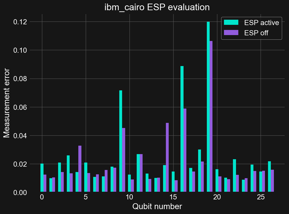
By eye we can see that the cyan bars are typically longer than the corresponding purple bars, qualitatively signaling that ESP readout gives worse measurement errors than those with it disabled. Let us look at the mean values for these error rates:
1-np.mean(esp_fids, axis=1)
array([0.0256358 , 0.02191749])
We see that the average error rate is indeed higher when using ESP than without. This is somewhat disappointing given that ESP is on by default here. However, this is just one system. Perhaps trying another gives different results. Here is data obtained on ibmq_perth using the same manner as above:
perth_esp_fids = [np.array([0.97066429, 0.97649286, 0.97842857,
                            0.98060714, 0.96941429, 0.9735, 0.98295714]),
                  np.array([0.98272143, 0.97831429, 0.97732857,
                            0.98332143, 0.98175714, 0.98055714, 0.99046429])
                 ]
fig, ax = plt.subplots()
ax.bar(np.arange(7), 1-perth_esp_fids[0], width=0.33, label='ESP active')
ax.bar(np.arange(7)+0.33, 1-perth_esp_fids[1], width=0.33, label='ESP off')
ax.legend()
ax.set_xlabel('Qubit number')
ax.set_ylabel('Measurement error')
ax.set_title('{} ESP evaluation'.format('ibm_perth'));
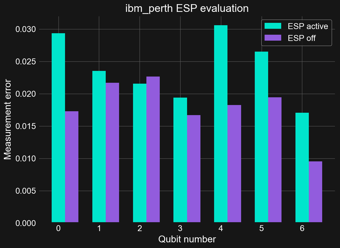
Again we see that ESP readout is worse than the standard readout method. Perhaps this is why it is enabled on only a few systems; there is no value in doing ESP readout on the latest IBM Quantum systems.