Choosing the best Qiskit swap mapper¶

One of the most important (perhaps the most important) steps when compiling quantum circuits for architectures with limited connectivity is swap mapping. If a requested two-qubit gate cannot be implimented directly on hardware, the states of the corresponding qubits must be swapped with those of their neighboors until the states reside on qubits where a two qubit gate is supported. Swap gates are expensive, equal to three CNOT gates, and therefore moving qubit states around using the fewest number of swap gates is desireable. Unfortunately, directly computing the minimum number of swap gates is NP-complete, and heuristics need to be developed that come close to the ideal solution while scaling favorably with the number of qubits.

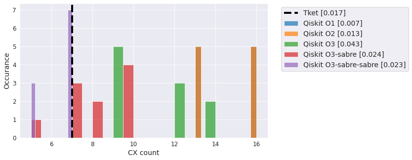
Qiskit supports a variety of swap mappers and other optimization settings, and how to best set these options is important for getting high-fidelty results. Additionally, there are other Qiskit compatible compilers out there that should also be evaluated. To this end, here we look at a selection of circuits compiled with various Qiskit compiler settings, as well as those produced with the Cambridge Quantum Computing (CQC) Tket compiler. We will investigate the performance of these methods in terms of both number of CNOT gates in the output, as well as the associated runtimes. Because Qiskit swap mappers are stochastic, we will run each one several times and plot the distributions of results.

Summary of results¶

When using the native Qiskit transpiler in general it is best to first try the following settings:

transpile(circuits, backend, optimization_level=3,
          layout_method='sabre', routing_method='sabre')

Additionally, because of the stochastic nature of the Qiskit swap mappers, ideally one should transpile the same circuit multiple times and select the one with the lowest number of CNOT gates in it. Alternatively one can get good results using the CQC Tket compiler via:

tk_qc = qiskit_to_tk(qc)
tk_backend.default_compilation_pass(2).apply(tk_qc)
tk_to_qiskit(tk_qc)

The Tket mapper is deterministic and thus only needs to be run once. It does appear to slow down at larger qubit counts when compared to the runtime of the Qiskit compiler.

Frontmatter¶

Import the needed libraries.

import time
import numpy as np
from qiskit import *

import matplotlib.pyplot as plt
import seaborn as sns
sns.set_style('darkgrid')

Load up some predefined circuits.

from qiskit.circuit.library import QuantumVolume, EfficientSU2, TwoLocal, QFT

To get the CQC Tket compiler and Qiskit interoperability on needs to first pip install pytket. Then we can load up the necessary IO and compiler routines.

from pytket.extensions.qiskit import qiskit_to_tk, tk_to_qiskit, IBMQBackend

Tket requires loading backends from the IBM Quantum provider. Thus we cannot use mock backends here. So we load up our IBM Quantum account and a provider.

IBMQ.load_account()
provider = IBMQ.get_provider(group='deployed')

Define the bechmarking functions¶

Here we define a couple of functions for benchmarking. First we need a way of compiling circuits via Tket and obtaining the CNOT gate count and the time it took (not including Tket <-> Qiskit conversion time). Second we need a similar routine for compiling in Qiskit. This is where things get tricky as there are a myriad of compiling combinations in Qiskit. Here we look at a few combinations. Namely we will try to compile at all the non-trivial optimization levels: 1 (default), 2, and 3. Additionally, we will turn on Sabre swap mapping, and then look at both Sabre initial layout and routing (here called “sabre-sabre”). Due to the stochastic nature of the swap mappers in Qiskit we will run each a couple of times and collect statistics. This is not really cheating as the compilation can be done in parallel. Finally, we make the primary user callable function compiler_benchmark that runs everything for us, and makes a nice plot.

def pytket_run(qc, tk_backend):
    """Get compling results for a given circuit and Tket backend.
    
    Parameters:
        qc (QuantumCircuit): The circuit.
        tk_backend (TketBackend): A Tket backend instance.
        
    Returns:
        int: Number of CNOT gates in compiled circuit.
        float: Compilation time.
    """
    tk_qc = qiskit_to_tk(qc)
    st = time.perf_counter()
    tk_backend.default_compilation_pass(2).apply(tk_qc)
    ft = time.perf_counter()
    return tk_to_qiskit(tk_qc).count_ops()['cx'], ft-st

def qiskit_run(qc, backend):
    """Get compling results for a given circuit and backend.
    
    Parameters:
        qc (QuantumCircuit): The circuit.
        backend (IBMQBackend): An IBM Quantum backend instance.
        
    Returns:
        list: Number of CNOT gates in compiled circuits.
        list: Best compilation times.
    """
    qk_cx_count1 = []
    qk_cx_count2 = []
    qk_cx_count3 = []
    qk_cx_count3l = []
    qk_cx_count3s = []

    qk_time1 = []
    qk_time2 = []
    qk_time3 = []
    qk_time3l = []
    qk_time3s = []
    for kk in range(10):
        st = time.perf_counter()
        qk_cx_count1.append(transpile(qc, backend,
                                      optimization_level=1).count_ops()['cx'])
        ft = time.perf_counter()
        qk_time1.append(ft-st)
        st = time.perf_counter()
        qk_cx_count2.append(transpile(qc, backend,
                                      optimization_level=2).count_ops()['cx'])
        ft = time.perf_counter()
        qk_time2.append(ft-st)
        st = time.perf_counter()
        qk_cx_count3.append(transpile(qc, backend,
                                      optimization_level=3).count_ops()['cx'])
        ft = time.perf_counter()
        qk_time3.append(ft-st)
        
        st = time.perf_counter()
        qk_cx_count3l.append(transpile(qc, backend, optimization_level=3,
                                       layout_method='sabre',
                                       ).count_ops()['cx'])
        ft = time.perf_counter()
        qk_time3l.append(ft-st)
        
        st = time.perf_counter()
        qk_cx_count3s.append(transpile(qc, backend, optimization_level=3,
                                       layout_method='sabre',
                                       routing_method='sabre').count_ops()['cx'])
        ft = time.perf_counter()
        qk_time3s.append(ft-st)

    return [qk_cx_count1, qk_cx_count2,
            qk_cx_count3, qk_cx_count3l,
            qk_cx_count3s], [np.min(qk_time1), np.min(qk_time2),
                             np.min(qk_time3), np.min(qk_time3l),
                             np.min(qk_time3s)]

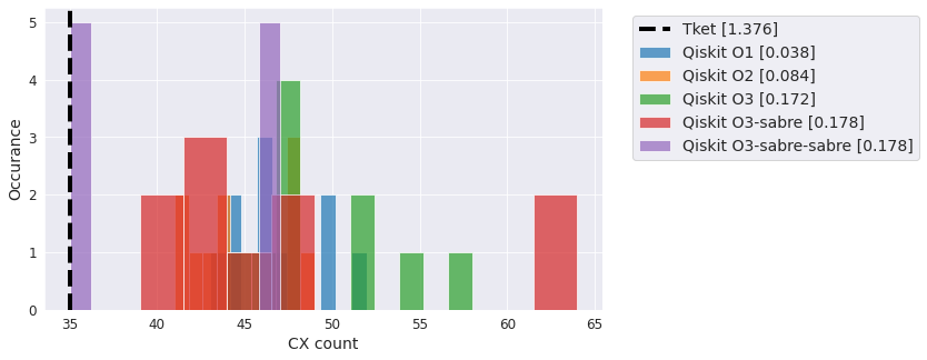
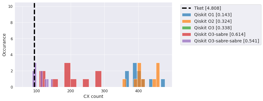
def compiler_benchmark(circuit, backend):
    """Benchmarks a circuit on the target backend and plot
    the results.
    
    Parameters:
        circuit (QuantumCircuit): The circuit to benchmark.
        backend (IBMQBackend): The target system
    """
    tk_backend = IBMQBackend(backend.name(), group='deployed')
    
    tk_cx_count, tk_time = pytket_run(circuit, tk_backend)
    qk_counts, qk_times = qiskit_run(circuit, backend)
    
    fig, ax = plt.subplots(figsize=(9,5))
    ax.hist(qk_counts[0], label='Qiskit O1 [{}]'.format(np.round(qk_times[0],3)), alpha=0.7)
    ax.hist(qk_counts[1], label='Qiskit O2 [{}]'.format(np.round(qk_times[1],3)), alpha=0.7)
    ax.hist(qk_counts[2], label='Qiskit O3 [{}]'.format(np.round(qk_times[2],3)), alpha=0.7)
    ax.hist(qk_counts[3], label='Qiskit O3-sabre [{}]'.format(np.round(qk_times[3],3)), alpha=0.7)
    ax.hist(qk_counts[4], label='Qiskit O3-sabre-sabre [{}]'.format(np.round(qk_times[4],3)), alpha=0.7)
    ax.axvline(tk_cx_count, color='k', linewidth=4, linestyle='--',
               label='Tket [{}]'.format(np.round(tk_time, 3)))
    ax.set_xlabel('CX count', fontsize=14)
    ax.set_ylabel('Occurance', fontsize=14)
    ax.tick_params(axis='both', labelsize=12)
    ax.legend(fontsize=14, bbox_to_anchor=(1.04,1), loc="upper left")

5Q-T tests¶

Here we run tests on a 5Q system with a “T”-shaped coupling map. This is a bit more interesting than a linear coupling when it comes to figuring out swaps. The Quito system has such a layout.

backend = provider.backend.ibmq_quito

GHZ / BV circuit¶

A commonly used test circuit where all CNOT gates require a control or target on a single qubit.

qc = QuantumCircuit(5)
qc.h(0)
qc.cx(0, range(1, 5))

<qiskit.circuit.instructionset.InstructionSet at 0x7f3bed0bcd30>

compiler_benchmark(qc, backend)

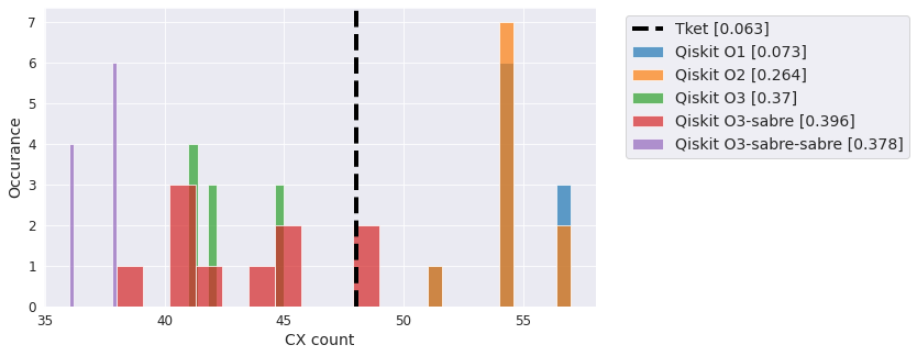
../../_images/2021-10-31-best_swap_mapper_qiskit_19_0.png

QV¶

The standard “quality” metric circuits. Results can vary (sometimes dramatically) based on generated circuit.

qc = QuantumVolume(5)

compiler_benchmark(qc, backend)

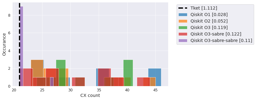
../../_images/2021-10-31-best_swap_mapper_qiskit_22_0.png

Efficient SU2 - linear¶

An ansatz circuit with linear entanglement profile.

qc = EfficientSU2(5, entanglement='linear')

compiler_benchmark(qc, backend)

../../_images/2021-10-31-best_swap_mapper_qiskit_25_0.png

Efficient SU2 - full¶

Same thing as above but with full entanglement.

qc = EfficientSU2(5, entanglement='full')

compiler_benchmark(qc, backend)

../../_images/2021-10-31-best_swap_mapper_qiskit_28_0.png

Two-local linear¶

Another flavor of ansatz with linear entanglement and several repeated layers.

qc = TwoLocal(5, 'ry', 'cx', 'linear', reps=5)

compiler_benchmark(qc, backend)

../../_images/2021-10-31-best_swap_mapper_qiskit_31_0.png

QFT¶

The Quantum Fourier Transformation (QFT). Also used a lot in benchmarking.

qc = QFT(5)

compiler_benchmark(qc, backend)

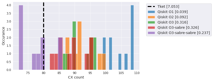
../../_images/2021-10-31-best_swap_mapper_qiskit_34_0.png

20Q tests¶

Here we expand or circuits to 20 qubits and look at compiling on a 27qubit Falcon heavy-hex topology.

backend = provider.backend.ibmq_mumbai

tk_backend = IBMQBackend("ibmq_mumbai", group='deployed')

GHZ / BV circuit¶

A commonly used test circuit where all CNOT gates require a control or target on a single qubit.

qc = QuantumCircuit(20)
qc.h(0)
qc.cx(0, range(1, 20))

<qiskit.circuit.instructionset.InstructionSet at 0x7f3be8804fa0>

compiler_benchmark(qc, backend)

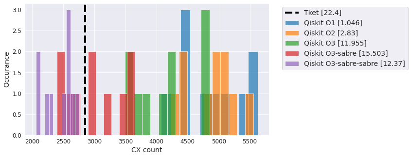
../../_images/2021-10-31-best_swap_mapper_qiskit_40_0.png

QV¶

The standard “quality” metric circuits. Results can vary (sometimes dramatically) based on generated circuit.

qc = QuantumVolume(20)

compiler_benchmark(qc, backend)

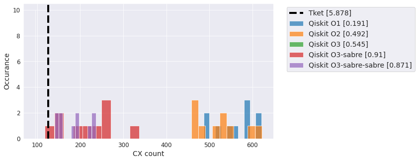
../../_images/2021-10-31-best_swap_mapper_qiskit_43_0.png

Efficient SU2 - linear¶

An ansatz circuit with linear entanglement profile.

qc = EfficientSU2(20, entanglement='linear')

compiler_benchmark(qc, backend)

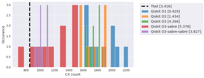
../../_images/2021-10-31-best_swap_mapper_qiskit_46_0.png

Efficient SU2 - full¶

Same thing as above but with full entanglement.

qc = EfficientSU2(20, entanglement='full')

compiler_benchmark(qc, backend)

../../_images/2021-10-31-best_swap_mapper_qiskit_49_0.png

Two-local linear¶

Another flavor of ansatz with linear entanglement and several repeated layers.

qc = TwoLocal(20, 'ry', 'cx', 'linear', reps=5)

compiler_benchmark(qc, backend)

../../_images/2021-10-31-best_swap_mapper_qiskit_52_0.png

QFT¶

The Quantum Fourier Transformation (QFT). Also used a lot in benchmarking.

qc = QFT(20)

compiler_benchmark(qc, backend)

../../_images/2021-10-31-best_swap_mapper_qiskit_55_0.png

Version information¶

from qiskit.tools.jupyter import *
%qiskit_version_table

/home/paul/miniconda3/envs/qiskit/lib/python3.9/site-packages/qiskit/aqua/__init__.py:86: DeprecationWarning: The package qiskit.aqua is deprecated. It was moved/refactored to qiskit-terra For more information see <https://github.com/Qiskit/qiskit-aqua/blob/main/README.md#migration-guide>
  warn_package('aqua', 'qiskit-terra')

Version Information

Qiskit Software	Version
`qiskit-terra`	0.18.3
`qiskit-aer`	0.9.1
`qiskit-ignis`	0.6.0
`qiskit-ibmq-provider`	0.17.0
`qiskit-aqua`	0.9.5
`qiskit`	0.31.0
`qiskit-optimization`	0.2.0
System information
Python	3.9.7 \| packaged by conda-forge \| (default, Sep 29 2021, 19:23:11) [GCC 9.4.0]
OS	Linux
CPUs	4
Memory (Gb)	62.73820495605469
Sun Oct 31 06:14:50 2021 EDT

pytket does not have any version (__version__) information. So you will just have to trust me that it is version 0.16.0

Dynamic Bernstein-Vazirani using mid-circuit reset and measurement Comparison of Falcon R5 processors verse R4

31 October 2021

Recent Posts

Archives

Choosing the best Qiskit swap mapper¶

Summary of results¶

Frontmatter¶

Define the bechmarking functions¶

5Q-T tests¶

GHZ / BV circuit¶

QV¶

Efficient SU2 - linear¶

Efficient SU2 - full¶

Two-local linear¶

QFT¶

20Q tests¶

GHZ / BV circuit¶

QV¶

Efficient SU2 - linear¶

Efficient SU2 - full¶

Two-local linear¶

QFT¶

Version information¶

Version Information